Categories
Olympic Park

London Olympic Park Construction

Last weekend I cycled around the perimeter of the building site that will be the Olympic Park in 2012. It’s a big site – over 9km all the way around.

Here’s some photos I took – click through to the Flickr pages for some slightly pithy commentary to go along with them:

Direct link to the photo set.

Categories
Mashups OpenLayers OpenStreetMap

Accuracy vs Completeness: OSM vs Meridian 2

[Updated x2] Yesterday’s Ordnance Survey OpenData launch has provided the OpenStreetMap community with a potentially rich set of data to use to complete the map of Great Britain. OpenStreetMap’s accuracy and detail is generally excellent, however a problem which is (very arguably) more important than either accuracy or detail, in a map is that some parts of the country are substantially incomplete.

It’s not that the data quality is poor, it’s that someone with a GPS (or a satellite photo) has never been to that part of the country to gather the data in the first place. There are still significant parts of Scotland and Northern England which have many missing roads. The NPE (out-of-copyright) maps have been useful in starting to fill out these sections, but there’s always going to be a roads missing from a 60-year-old (or older) map.

So, the OS datasets could be very useful. Perhaps the most interesting of the datasets is Meridian 2, it is a vector dataset covering the whole country. One thing that needs to be watched out for though is that Meridian (which is a “complete” dataset of the country) is relatively inaccurate Pixellation or resolution isn’t a problem, it being vector based – but data is quite simplified.

I’ve built a mashup which allows direct comparision of the Meridian and OSM data for Great Britain. I’ve added in most of the available layer files that come with the Meridian package that has been released as part of the OS OpenData initative. The only two areal ones I’ve added are for woodland areas and lakes – everything is linear. I’ve added in labels for the roads and rivers, but no boundaries or point features, at this stage.

You can access the mashup here [now offline] (N.B. Not tested in IE so will probably break horribly in it.) Zooming in reveals the relative coarseness of the Meridian data – although crucially it is “substantially” complete for all but the smallest of roads, for the whole of the UK – not just for the major cities where the OSM contributors mostly live!

Completeness
In the pictures below, the “solid”, thinner roads are Meridian and the fatter roads with “borders” are OSM.

Spot the missing roads in Meridian around Leytonstone in East London [Update 1 – Some sections of motorway are missing from my rendering but are present in the data – it is possible this problem extends to smaller roads too so take these screenshots with a pinch of salt]:

…but go further out of London, and it doesn’t look so good for OSM:

Interestingly, the Park Estate in central Nottingham is missing entirely from Meridian:

The Park Estate is a private estate and the roads are not maintained by the council – this might have something to do with it. I’ll be running around the Park Estate next weekend.

Accuracy
[Update 2 – Meridian is not intended to be used at scales larger than 1:50000, as per its documentation, so I shouldn’t really be comparing it with OSM which generally is based on data recorded at larger scales. So, bear in mind these screenshots are all larger than 1:50000 scale.] It’s difficult to authoritatively judge the relative accuracies of the two datasets without getting out on the streets or looking at aerial imagery – but you can infer a basic measure of accuracy by looking at how roads “wiggle” – or, in the case of the Mayfair squares below, how Meridian converges the square to a point:

Detail
A little unfair to compare the two here, as Meridian 2 was always meant to be a medium-scale dataset, whereas OSM can be all things to all people!

The tiles that make up the imagery are generated on demand (and cached for subsequent use) so may run slowly. You’ll need to zoom in quite a long way before all the features get added to the map. Use the slider on the top left to fade between the OSM and Meridian layers.

The images are derived from Ordnance Survey data © Crown copyright and database right 2010 and OpenStreetMap data which is CC-By-SA OSM and contributors.

Categories
Data Graphics Technical

Forests of Great Britain

From the OS OpenData’s Meridian 2 dataset, which was released under a free licence today, here is the extent of forest cover across Great Britain – there is a dedicated polygon shapefile within the distribution showing just this:

As a general rule for orienteering, areas with good forest cover have the best orienteering maps. Scotland and Wales beat England hands down for cover, although Surrey’s doing not too badly at all. The rule doesn’t always hold though – there’s a big patch near Cambridge – more so, it appears than the Lake District, but the latter is considerably finer for orienteering in.

The map contains Ordnance Survey data © Crown copyright and database right 2010.

Categories
Mashups Technical

OS OpenData is here

It’s the first of April – but it’s not an April Fool – lots of Ordnance Survey medium-scale data has been released today, under a licence compatible with Creative Commons’ Attribution, i.e. you can do what you like with it as long as you attribute and don’t misrepresent the data source.

The best mirror for the data I’ve found is at MySociety – the OS’s own servers have been apparently overloaded since the release went live.

The first use I’ve made of the data is taking the “CodePoint Open” set of postcodes and locations, I’m now using this data as the postcode lookup for OpenOrienteeringMap. If you type in a UK postcode there, it should now take you to exactly the right place. Before, the lookup was using NPEmap data, which was pretty good in general, but someone did spot some glaring errors when they were using it, coincidently, yesterday.

The attribution statement, by the way, can be seen by mousing over the “Jump to Postcode” text.

Categories
OpenStreetMap

Scottish Popular Edition Tracing for OSM

The provision of free-for-any-use spatial data for the UK may be changing dramatically on April 1 with the anticipated release of some Ordnance Survey mid/small-scale mapping and data for unrestricted use.

Until then, the only Ordnance Survey maps that have been able to be used to derive data from for the OpenStreetMap project in its bid to complete coverage in the UK, are those that are more than 50 years old and therefore not protected by Crown Copyright.

Scans of such maps, generally the New Popular Edition from the 1940s/50s, have been available for some time now – the scans were originally done for the NPEmap project (gathering copyright-free postcodes by asking people to geolocate them to the maps) and then were orthogonalised and reprojected from the British National Grid into the “Web Mercator” projection used by Google Maps, the “standard” OpenStreetMap website and numerous other online “slippy” maps.

Scotland wasn’t included at the time, partly because the maps were sourced differently. After consultation with the owners of the scans, I’ve taken the imagery, rectified, reprojected, stitched and tiled it using TimSC’s warp-gbos tools, so that it can now be used to trace Scottish data.

The source maps are at 1:63360 scale (one inch to a mile) and typically there remains an error of around 10m – up to 30m in some places, and of course more where the source map was drawn slightly incorrectly. So the imagery isn’t particularly useful for detailed mapping – particularly in cities which have seen significant growth in the last 50-80 years since the maps were made. However they are very useful for completing the rural road network, town and village names and natural features (hills, rivers) that are unlikely to have changed significantly recently – the low-res Landsat imagery can be used to show the presence of more recent forests or reservoirs.

In the above example, it would not be unreasonable to assume the path here still exists, and add it in – citing the source. You could also add the cliff, and reshape the lochs slightly from their current jagged Landsat-derived image. Adding in names for the hills and the lochs are also a definite benefit, although these old maps tend to have the Anglicised versions of names – newer editions of OS mapping for the Highlands of Scotland tend to use more authentic Scottish-Gaelic names. (Not an issue in this particular example, just north of Slioch in the Great Wilderness, as all the names on the map are in Gaelic.)

You can see the map tiles while editing OpenStreetMap data in Potlatch for Scotland, by selecting “UK Historic: Scotland” in the Potlatch preferences pane. They are available to zoom 15, although zooms 14/15 are simply smoothly interpolating pixels. The tiles are hosted on a computer under my desk here at UCL. There are better quality and higher resolution scans of more recent maps for some parts of Scotland, information about these is . The main advantage of the Scottish Popular Edition tiles over using just these they offer substantially complete coverage of Scotland.

(Strictly, some of the areas are using newer mapping which is still more than 50-years old, but is part of more recent editions than the Scottish Popular Edition).

So, the main benefit – having a map with full coverage of Scotland which can be traced from for OpenStreetMap – may be diminished, if a useable equivalent appears shortly which is only a few years out of date (i.e. Ordnance Survey Landranger/Explorer), but for now, they are still a useful source of base data.

If you just want to look at the mapping rather than editing them, you can see them here on my own site, or here on the NPEmap project.

Categories
Leisure

Parkrun – The Video

Here’s a brilliantly produced video showing what parkrun is all about.

It’s shot on location in (I think) Bushy Park in south-west London. Plenty of shots of the verdant park and the wildlife, as well as the runners.

Categories
OpenStreetMap

UK Mapping Priority Areas – by Bus Stop?

The OSM wiki has a list of UK Mapping Priority areas, where there are a presumed substantial number of missing roads which need to be mapped. These can then get mapped at a mapping party. The probable introduction of a freely-derivable “complete” set of Ordnance Survey road data in ten days time may mitigate the need to do such first-step mapping, but for now there are many areas in the UK which could do with some on-the-ground data gathering.

As an alternative way of identifying such areas, I developed the “Lonely Buses” map. As an extension to this, I’ve now created a “top 50” list of areas that have the most number of bus-stops away from roads, i.e. areas with probable missing roads. You can see this list here. A basic form of reverse geo-coding is used to assign a name to each tile.

The list is automatically updated weekly. It is flawed in that it considers each “tile” exclusively, so if a town is split in half by tile edges, it will appear twice and lower down the list, compared to a similarly incomplete town being in the middle of its respective tile.

Looks like the Newcastle area is the No. 1 target area (within areas which have the government bus-stop dataset imported.)

Andover has a mapping party planned for mid-May and is currently No. 39 on the list. If you are in the area, sign up!

Categories
OpenStreetMap Technical

Map Adornments with Cairo

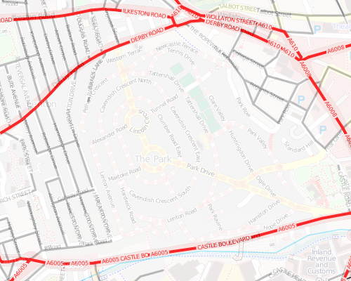
For my OpenOrienteeringMap service, I have a added PDF creation facility, which produces a map, ready to print, with a title, north arrow, club logo and link back to the website.

The map itself is rendered in Mapnik, which uses Cairo, using Python and the pycairo bindings. To add the adornments, I’ve also made use of these bindings, and use them at the same time.

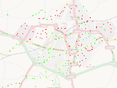
The adornments are shown above highlighted in yellow, and the purple control circles and numbers are also added directly using Cairo, rather than being rendered as geospatial objects in Mapnik. This blog post concentrates on the ones at the top of the sheet.

Here’s part of the Python script used to produce the PDF. S2P is a constant used to convert from metres (i.e. map units) to points (i.e. screen/paper units) and its value is 72/0.0254 (72 points per inch, 1/2.54 inches per cm).

I’ve generally use capitals for the names for the various positioning values, with a sort of naming convention – “W” is width, “WM” is west (i.e. left) margin. For example, ADORN_L_W is the width of the logo adornment, in metres. The “surface” sheet is made up of various “contexts” – in effect content boxes, which are positioned and scaled onto the surface, and filled with the content.

We need to import some modules:

import tempfile
import mapnik
import cairo
import urllib

Firstly, set up the PDF sheet, or “surface”, specifying its size:

file = tempfile.NamedTemporaryFile()
surface = cairo.PDFSurface(file.name, PAPER_W*S2P, PAPER_H*S2P)

It’s important to specify the sizes accurately so that printers will print without trying to reduce the PDF, so rendering the scale inaccurate. For example, A4 landscape needs to have a PAPER_W of exactly 0.2970 and PAPER_H of 0.2100.

Then set up the map element – note Mapnik requires integers for the widths and heights:

map = mapnik.Map(int(MAP_W*S2P), int(MAP_H*S2P))
mapnik.load_map(map, styleFile)
map.zoom_to_box(cbbox)

Create a context on the surface to draw the map onto, and shift it to allow for margins on the page.

ctx = cairo.Context(surface)
ctx.translate(MAP_WM*S2P, MAP_NM*S2P)
mapnik.render(map, ctx)

Then, just add each adornment in the right place. First the title – the text has been supplied in the URL so is decoded first:

text = urllib.unquote(title)

Then, write the title onto the surface using show_text. Obviously, the server needs to have the fonts installed – I was using Deja Vu Sans initially, but Arial is used for the “regular” Street-O maps that I’m mimicing, so I installed the Microsoft Truetype Core Fonts for Linux:

ctx = cairo.Context(surface)
ctx.select_font_face("Arial Black", cairo.FONT_SLANT_NORMAL, cairo.FONT_WEIGHT_NORMAL)
ctx.set_font_size(24)
ctx.translate(MAP_WM*S2P, (MAP_NM-ADORN_T_SM)*S2P)
ctx.show_text(text)

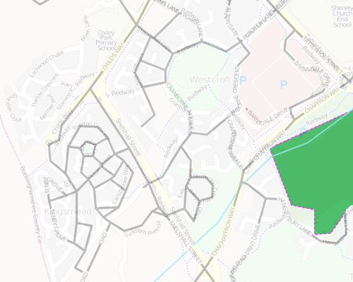
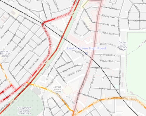
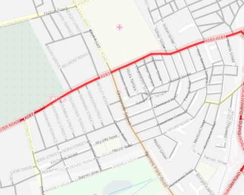
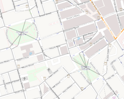
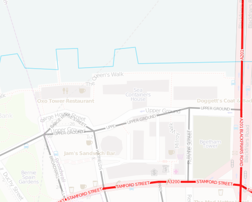
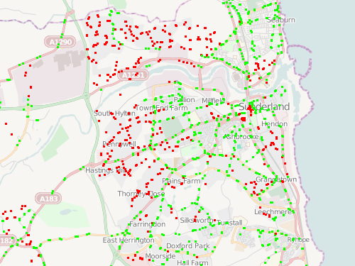
The image above – and the ones below – are shown at 150% of their actual size on screen.

Now to add a scale caption:

ctx = cairo.Context(surface)
ctx.select_font_face("Arial", cairo.FONT_SLANT_NORMAL, cairo.FONT_WEIGHT_NORMAL)
text = "Scale 1:" + str(scale)
ctx.set_font_size(14)
width = ctx.text_extents(text)[4]
ctx.translate((MAP_WM+MAP_W)*S2P-width-(ADORN_A_W+ADORN_L_W)*S2P, (MAP_NM-ADORN_S_SM)*S2P)
ctx.show_text(text)

..and below it, a scalebar and indicator:

ctx = cairo.Context(surface)
ctx.select_font_face("Arial", cairo.FONT_SLANT_NORMAL, cairo.FONT_WEIGHT_NORMAL)
scaleBarMetres = 500
if scale < 10000:
    scaleBarMetres = 200
text = str(scaleBarMetres) + "m"
ctx.set_font_size(7)
width = ctx.text_extents(text)[4]
barCaptionX = (MAP_WM+MAP_W-(ADORN_A_W+ADORN_L_W))*S2P-width
ctx.translate(barCaptionX, (MAP_NM-ADORN_S_SM)*S2P)
ctx.show_text(text)

..the scalebar itself, making use of stroke:

ctx.set_line_width(0.5)
scaleBarW = scaleBarMetres/float(scale)
ctx.move_to((-scaleBarW-ADORN_S_PADDING)*S2P, 0)
ctx.rel_line_to(0, -ADORN_S_LARGETICK*S2P)
ctx.rel_line_to(0, ADORN_S_LARGETICK*S2P)
ctx.rel_line_to(scaleBarW*S2P/2, 0)
ctx.rel_line_to(0, -ADORN_S_SMALLTICK*S2P)
ctx.rel_line_to(0, ADORN_S_SMALLTICK*S2P)
ctx.rel_line_to(scaleBarW*S2P/2, 0)
ctx.rel_line_to(0, -ADORN_S_LARGETICK*S2P)
ctx.stroke()

The north-arrow is done in a similar way. close_path is used to create a proper triangle, with no “ends” that might result in ugly capping effects. fill makes it solid.

ctx = cairo.Context(surface)
ctx.translate((MAP_WM+MAP_W-ADORN_L_W)*S2P-width, CONTENT_NM*S2P)
ctx.set_line_width(1)
ctx.move_to(0, 0)
ctx.line_to(0.001*S2P, 0.002*S2P)
ctx.line_to(-0.001*S2P, 0.002*S2P)
ctx.close_path()
ctx.fill()

The “N” below the arrow is also drawn with lines, but using round line joins and line caps to produce a smooth letter.

ctx.move_to(0, 0.001*S2P)
ctx.line_to(0, 0.008*S2P)
ctx.stroke()
ctx.set_line_join(cairo.LINE_JOIN_ROUND)
ctx.set_line_cap(cairo.LINE_CAP_ROUND)
ctx.move_to(-0.001*S2P, 0.005*S2P)
ctx.rel_line_to(0, -0.002*S2P)
ctx.rel_line_to(0.002*S2P, 0.002*S2P)
ctx.rel_line_to(0, -0.002*S2P)
ctx.stroke()

Finally, a logo is added. This is a bit trickier – the logo is a PNG, but the surface is a PDF. The way I got around this is to create a temporary ImageSurface and then switch the surface that the context is on – the graphic also gets appropriately scaled:

logoSf = cairo.ImageSurface.create_from_png(home+"/logo.png")
ctx = cairo.Context(surface)
width = logoSf.get_width()*ADORN_L_SCALE
ctx.translate((MAP_WM+MAP_W)*S2P-width, CONTENT_NM*S2P)
ctx.scale(ADORN_L_SCALE, ADORN_L_SCALE)
ctx.set_source_surface(logoSf , 0, 0)
ctx.paint()

Finally, putting it all together:

surface.finish()
return file

Categories
OpenStreetMap

On Lonely Buses and Orphaned Bus Stops

Contributors to OpenStreetMap in the UK have been gradually importing in the NaPTAN dataset of the locations of bus stops (amongst other things).

Many, but not all, of the local authority areas, have now had their bus stops imported in to the OpenStreetMap database in this way. These, and the other areas, also have bus stops shown that have been manually added by contributors based on ground observations.

In areas where the roads have not been added into OSM (and there are still plenty such areas, where there is no accurate aerial imagery to trace from, or contributors on the ground with GPS) the bus stops will appear disconnected from any road on the map. Large numbers of these “orphaned” bus stops in an area are indicative that key roads or even whole villages and towns are missing from the map.

To aid discovery of such roads and towns, I’ve created a simple visualisation. Bus stops appear as green dots if they are within around 20m of any highway (this does include cycle paths, paths and railways, but in general if these features are present, nearby roads would be too). Stops that are further away are shown as red dots.

The visualisation can be seen here. The mapnik stylesheet used is here (XML) – Mapnik 0.7.0+ is required because of the !bbox! usage, and the generic entity stylesheets used in OSM/Mapnik are also referenced.

The tiles are generated directly from my copy of the OpenStreetMap “planet” database, using Mapnik to call PostGIS with a spatial query. The process of calculating the bus stop statuses is reasonably CPU-intensive – for each bus stop, a buffer around the stop is created and then line-in-polygon tests are done on all roads in the area using a spatial index. PostGIS makes the process straightforward – ST_DWithin is used for the buffering, and ST_Intersects is used separately on the stops and highways to restrict the search to the local area.

To reduce the complexity of the query, the cut-off distance actually varies slightly – the coordinate reference system used is “metres” in EPSG 900913 – the so-called “Google” projection. The “metres” are only 1m long at the equator – away from it, they are shortened by a factor of cosine of the latitude, so for UK latitudes, 30 EPSG 900913 metres are equivalent to between 14 and 20m, decreasing as you travel north.

The results show some key towns in need of more roads, such as Cleethorpes, Kidderminster and Thetford, while much of the town-to-town network in SE England is pretty good. The process does assume the bus stop locations are correct, which is not necessarily the case, and also for very wide roads, the bus stops in real life may be further away than 20m from the road centreline, and so incorrectly shown on the visualisation.

Basingstoke is looking pretty good:

But nearby Andover needs more mapping:

In places, the density and linearity of the orphaned bus-stops means that, in theory, a road could be added to OSM based solely on the pattern of stops in these places.

Try it out here [now offline].

Categories
Technical

A Google Streetview History

Inspired by Alex – all the places I’ve ever lived:

Google’s UK streetview coverage isn’t quite ubiquitous – a couple of the images are snapped looking across fields from the nearest main road, and one of the images is pointing in the correct direction, but the house is completely hidden by all the trees in that general area.

The New York one should be pretty easy to spot, as well as my move to London and its terraced housing. The last picture is of my parent’s new house – the Google camera seems to have fallen onto its side when driving down this particular steep and twisty road.