Categories
London Technical

Me, Geolocated on Twitter

tweets_london

I was prompted by the excellent Twitter Tongues map, where geolocated tweets in London (including mine, and those from hundreds of thousands of others) were mined by Ed Manley over the summer, and then mapped by James Cheshire, to see where I had left my own Twitter footprint.

Many people would probably be quite alarmed to learn that the data, on the exact locations they have tweeted at – if they’ve allowed geolocation – is freely accessible to anyone, not just themselves, through the Twitter API.

tweets_chancerylane

It’s a bit of a faff to get the data – Twitter is starting to rollout a “download my Tweets” option which may make the first few steps here easier – but here’s how I did it.

  1. I used the user_timeline call on the Twitter API, repeatedly, to pull in my last 3200 tweets (the maximum) in batches (“pages”) of 200. The current Twitter API (1.1) requires OAuth authentication – not of the person whose tweets you are mining, but simply yourself, so that rate limits can be correctly applied. Registering a dummy application on the Twitter gives access to OAuth credentials, and then using the OAuth tool generates a CURL string that can then be run – the result is put in a file ( > pageX.json), and I do this 16 times to get all 3200 tweets, using the count, page and include_rts parameters. For this particular case, I’m interested in the locations of my own account but – to stress again – you can do this for anyone else’s account, unless their account is protected and you are not a follower.
  2. The output is as various JSON files. Lacking a JSON parser, or indeed the skill, I had to do a bit of manual text processing. Those with a flexible JSON parser can therefore skip a few steps. I then merged together the files (cat *.json > combined.txt), and in a text editor, put a line break between each },{"crea and replaced ," with ,^" with the caret being an otherwise unused character.
  3. I opened up the file as a text file (not CSV!) in Excel and did a text-to-column on the caret. I then extracted three columns – the date/time, tweet text, and the first coordinates column that occurred. These were the 1st(A), 4th (D) and 28th (AB) columns. I did further find/replace and text-to-columns to remove the keys and quotes, and split the coordinates column into two columns – lat and long.
  4. I removed all the rows that didn’t have a lat/long location. Out of 3186 (14 less than 3200 due to deleted tweets) I had 268 such tweets. I also added a header row.
  5. I created a new Google Fusion Table on the Google Drive website, importing in the Excel file from the above step, and assigning the latter two columns to be a two-column location field.
  6. I marked the table as public (viewable with a link). This is necessary as Google doesn’t allow the creation of a map from a private file, except though a paid (business) account. The flip side of course is this gives Google themselves the right of access to the file contents, although I can’t imagine they are particularly interested in this one.
  7. Finally, I added a tab to the Google Fusion Table which was a map tab, and then zoomed in and around and took the screenshots below. The map is zoomable and the points clickable as normal. It should be possible to colour-code the dots by year, if the categories are set appropriately and the appropriate part of the datetime feed is reformatted appropriately in Step 3.

The whole process, including some trial-and-error, took a little over an hour – not so bad.

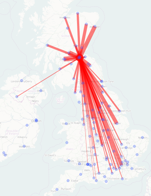
In the images above and below, you can see the results – 268 geolocated tweets over the course of two and a half years from my account – many of them precisely and accurately located.

tweets_nweurope

All screenshots from Google Maps.

Categories
Training

Evolving the Shoe, Evolving the Terrain

mizuno_wi9w

I occasionally receive the odd running-related press release, and got an interesting one from Mizuno recently, announcing a couple of new running shoes – the Wave Rider 16 and Wave Inspire 9 – the two being quite similar but with the latter being more of a support shoe and a fraction (10g) heavier.

The shoes look the part as you would expect, and are appropriately vividly coloured and styled – very much the trend these days, and why not – at this time of year, much of the time it’s dark when I’m running, and it makes sense to be as visible as possible.

Anyway I mention the shoes for three reasons.

Firstly I’m impressed that this is the 16th iteration of the Wave Rider shoe. Mizuno clearly know they are on to a good thing – not launching a new brand every year or so, but instead evolving a well known one. The average running shoe only lasts for 3-400 miles so a typical club runner might need to buy a new one twice a year. If the shoe is good, then the club runner will not want to change it for another brand if the old one is no longer available – they might just as easily change the manufacturer altogether, but they would much prefer to stick the name of the shoe that they know – shoes are the critical tool for a runner. So, give them what they want, and take the opportunity to refine it.

But you also need to keep new people discovering the manufacturer and brand, and also update the look to keep it looking new and relevant. So – relaunch it!

The second reason I mention is that I got a rather nice Mizuno freebie – which just happened to be a Wave Rider 15 – during the launch of an unrelated training shoe by them, earlier this year. Like the new shoes here, it wasn’t a subtle shoe – purple and lime green. When added to my red, white and blue running tops, the look is somewhat psychedelic. But it’s a very comfortable shoe and has become my current running shoe of choice. This is partly due to superstition – I started wearing my previous new shoe when I hadn’t fully recovered from an injury, and I put the resulting niggles down to the shoe and not my injury – d’oh. But it’s surprising just how superstitious you can be when it comes to injuries.

Anyway, long story short, I’ve been very pleased with my “v15” Wave Rider the last few months – I even took it to the Venice Street Race in November, although Venice was underwater at the time* so there was not much running involved, and it could well be the v16 that I end up getting next, when the current one wears out – or maybe there will even be a v17 by then? It looks like the Wave Riders will be evolving for a while yet.

The third reason is the that PR came with some photos, of runners running in the shoes, like you would expect. But the locations strongly reminded me of urban orienteering races. None of the running in the photos is taking place on roads, but instead they are along the seafront, through building courtyards, along garden paths – all the places where the best urban orienteering takes places. The campaign’s ad (short video – 30s) even includes the runner ascending some external stairs – very Barbican. You could easily imagine a control in each of these photos. In fact I very nearly doctored the photos to add one in the background. I don’t think Mizuno would have been too impressed at that though.

I’m planning a big urban orienteering race – in fact the second biggest standalone one in the world – next September. It might even be the biggest in the world next year, because the traditional incumbent, Venice, has got cancelled in 2013, after some concerns were raised during this year’s flooded race. Details of the race I’m planning will be up at the end of this month – all I can say for now is that it will have a distinctly watery feel to it. As the planner, I get to pick where the control sites go. And I’ll certainly be aiming to pick ones like the sorts shown in the photos here.

* Resulting in a rather saline shoe now. I’m not sure if it would survive a wash cycle.

mizuno_wi9m

Categories
Bike Share Conferences

Paris Workshop on Bike Sharing Systems

IMG_2856

I attended a one-day workshop last week, hosted by IFSTTAR’s GERI Animatic research group at École des Ponts ParisTech just east of Paris. The workshop was on Bicycle Sharing Systems, and as I have recently been working with a couple of colleagues, Dr Martin Zaltz-Austwick and Dr James Cheshire, on research relating to bicycle sharing data, and mapping the systems currently live in various cities around the world, I was keen to attend, particular as the agenda was packed with interesting sounding talks.

My rush-hour commute through Paris proved to be slightly more traumatic than planned (I wonder if Parisian visitors find London Underground stations as confusing as I find those on the Paris metro?) but I arrived at the École des Ponts ParisTech in time to hear the workshop organiser introducing the sessions. First up was Pierre Borgnat talking about network analysis of Lyon’s system. I had seen a paper by him on Lyon before, and the popularity and density of Lyon’s system has allowed for a rich and interesting dataset for mining and community detection. The community detection has been done using both spatial and temporal variables. Pierre’s thorough and technical treatment of the data was backed up with some excellent mapping of the data, which you can see above and below.

IMG_2859

Next up was Jon Froehlich. Jon’s talk was underpinned by a discussion of the different data sources and types available in the field. He focussed on temporal cluster analysis of the Barcelona bicycle sharing system (below) – a particularly interesting city for me as, along with London and Zurich, it is a case study for the EU project I have recently started working on, EUNOIA. Barcelona’s bicycle sharing system is not unlike London’s, in terms of its size, shape and usage characteristics – although the general downward slope of the city causes headaches for its operator. Jon gets bonus points for including not only a quote from this blog on his presentation, but Martin’s beautiful routed bike-flow animation for London, and Dr Jo Wood’s more recent bi-directional flow animation, again of London.

IMG_2887

Etienne Côme, from the hosting school, was next on, with an analysis of the biggest system (outside of China) of all – the Vélib in Paris. The Vélib is perhaps the holy grail of academic research in the field as its size, and Paris’s multiple commercial and residential zones, means that community and network analysis is likely to be eye-opening. Similar to Pierre, Etienne outlined eight detected communities, by looking at temporal variations in the origin-matrix between the 1200-odd stations on the Vélib network.

IMG_2914

After lunch, Vincent Aguilera was first on, with a switch away from bicycle sharing systems but showing some techniques that have potential for the field – Vincent looked at using mobile phone network data to detect station dwell times and true journey durations on a section of the RER metro in Paris. He compared this data with Twitter messages with appropriate hashtags (below), and the real-time running supplied by the operator on its website. The availability and structure of the cell-towers on the network allowed a direct comparison to be made – indeed, such data may actually be of better quality than that currently available at the operator’s disposal, allowing more fine-tuned operation and monitoring.

IMG_2925

Neal Lathia was next with a look at London’s system – specially effects caused by the addition of casual (i.e. non-key, non-member) availability in December 2010. The additional option did see some changes in the usages of certain docking stations. The comparison was done by clustering the network’s docking stations by time, before and after the transition, and then seeing which stations changed cluster. One of the main areas of change was in the very heart of London, around the Trafalgar Square area, suggesting a slight shift away from the (still dominating) railway station-based usage patterns.

IMG_2948

Fabio Pinelli’s talk was wide-ranging – it included system design, routing for Dublin’s (over)used system, a look at the reliability of the Vélib fleet.

IMG_2950

Finally, Francis Papon from the hosting school took a step back from the modern electronically managed bicycle sharing systems and mobile/social data sources, and looked at change in uses of urban cycling more generally. His dataset stretched over a hundred years, rather than the typically five-year maximum historical range that bicycle sharing systems have. A key trend is that in the largest French cities studied, including Paris, there is a recent (post-2000) renaissance in urban cycling usage, but this is not matched in many of the country’s smaller cities.

The workshop concluded with a general discussion of the research field to date and its direction. What was particularly interesting was that several bike sharing operators were in attendance, they were fully engaged with the academic research being carried out, asking questions but also revealing some nuggets of information about how the systems are rebalanced, relative costs of operations and why they thought some systems were more successful than others.

Hopefully there will be more such workshops in the future in Europe – with UCL CASA, Cambridge, City University London and LSHTM all involved in the field, maybe there should be one taking place in London next year?

Categories
Data Graphics London

A Periodic Table for London

Here is a webpage that uses my own CityDashboard API*, to build a Periodic-Table inspired “data artwork” of live London information, as a series of coloured square panels on a website. The squares update regularly with fresh information, and throb red (or blue) if there are particularly extreme values present.

As an artwork, it’s deliberately not 100% clear what it shows. A key on the bottom right will help a bit, but a degree of guesswork will be needed for some of the panels. With a bit of thought, almost all of the panels should be decipherable.

It’s a super-simple webpage. I’m using CSS3 for the animations – no Javascript used. The page is customised to be most relevant to the CASA office here in central London – the chosen weather station, bike share stands, air quality monitor and variable message road sign have been chosen accordingly. A more sophisticated version – which doesn’t currently exist but would be simple to do – would use a combination of the location information in the CityDashboard feeds, and the HTML5 geolocation functionality of many browsers, to show a version more relevant to where in London the viewer is.

As the page is so simple, it displays well on mobile browsers – on my iPhone, the webpage shows four panels on each row. On larger displays, it will rearrange appropriately. See the acknowledgements link on the page to see where the data’s coming from – the same sources as CityDashboard, including TfL, DEFRA, Yahoo! Finance and Mappiness, as well as CASA’s own sensors.

I created the piece for the ODI’s recent Data as Art installation competition – I didn’t win, but decided to do it anyway.

Live version here.

*Strictly, I’m using my Bike Share Map data for the individual docking station information – this could be easily added to the CityDashboard API in due course.

Categories
Data Graphics London Mashups

Update to CityDashboard CSV API & iPad Wall!

I’ve made some minor alterations to the CSV API for CityDashboard. The main changes are in the metadata rows (the top two) rather than the subsequent rows. Specifically, the top metadata row has now split out the description, source and source URL – which were previously rather messily combined into a bit of HTML – into three text fields; and the second metadata row now uses properly formatted names for value titles, i.e. including spaces, and units, for example “broken_pc” now becomes “% docks/bikes broken”.

The reason for these changes is to accommodate a new and exciting use of the API here at CASA – our lab hardware specialist has recently been hard at work building an “iPad wall” and one of the visualisations in it is of CityDashboard data. Here’s what the uncompleted – but operational – iPad wall looks like (source):

It’s a physical CityDashboard!

I also took the opportunity to fix a few bugs and typos – mainly just cosmetic, but including a pretty silly one for the Mappiness-sourced data that was over-reporting the true value by a large and variable amount. Entirely my fault. That will serve me right for doing a coding change during a colleague’s Ph.D viva drinks reception! I also handle temporarily unavailable source feeds a little better – they’ll now appear unavailable for one complete update cycle but it means the source server doesn’t get repeatedly hammered until it comes back up again.

Categories
Data Graphics London

The Electric Tube

[Update – An updated version of this is currently available as a limited edition A2 print.]

In six weeks time, London will have a second orbital railway. The Circle Line has been running for just over 100 years, and on 9 December will be joined by the latest addition to Transport for London (TfL)’s Overground network – a link between Clapham Junction in the south-west and Surrey Quays in the south-east. This means that the West London Line, North London Line, East London Line and South London Line will all be linked up (you won’t be able to travel 360 degrees on one train though – you’ll need to change at both Highbury & Islington and Clapham Junction, and often Willesden Junction, to complete a circuit). Should you travel around the complete loop, you’ll pass through areas as varied as Imperial Wharf, Dalston Junction, Whitechapel and Peckham Rye.

Anyway this was a tenuous excuse for me to produce a diagram – above – of London’s TfL-owned network – the Underground, the Overground, the DLR, Tramlink and the Cable Car. Click the graphic for a larger version. My starting principles for the diagram were concentric circles for the orbital sections of the Circle Line and the Overground network, and straight lines for the Central and Piccadilly Lines, with the latter two converging in the centre of the circles. I then squeezed everything else in. I realised that the Northern Line’s Bank branch passed the Circle Line three times so was going to need something special, so I added a sine wave for this section, and extended this north and south as much as possible.

The River Thames is on there – because any tube diagram doesn’t look correct without the river – and the diagram is topologically accurate – everything connects correctly, and features are in an approximately correct geographical position relative to their neighbours, but not to the diagram overall. Only stations that are designated intersections, or have connections with National Rail stations, are shown. I haven’t labelled anything. It’s art.

I was also thinking about physics when creating the diagram – specifically Feynman diagrams, bubble chamber traces, particle physics collisions, magnetic flow lines and electrical circuit diagrams (as was Beck himself). Hence why I’ve called it the Electric Tube.

The work was also inspired by the likes of Fransicso Dans (more) and Project Mapping, as well as of course the famous Official Tube Map. [Update – I’ve updated the map slightly to add in Tramlink and a few more connections.]

Categories
Orienteering

Urban Events – How Far Do People Travel?

Intrigued by a comment on the Nopesport forums suggesting that local clashes rather than a very major international clash were the thinking behind the scheduling of a future urban event, I thought I would do some analysis of how far people travel to races, using my stats database of results.

To do this, I’ve excluded (a) people listed with a club of “IND”, “None” or “” (probably local non-orienteers), (b) people in non-geographical clubs (e.g. RAFO, AROS), as it’s difficult to pinpoint where they travelled from, and (c) clubs with less than 100 runs in the 3 or so years the events database runs back for – this leaves 113 clubs, the largest being BOK with 8534 runs. The latter exclusion also excludes most foreign clubs, although a number do make it through – particularly Irish ones. I’ve also assumed that remaining people live in the centroid of their club’s area of influence – which is “guesstimated” by me based on the name of the club. I’ve also assumed that the event, put on by the club, also takes place in the centroid of that club’s area of influence.

Anyway, here’s where everyone* travelled from to get to the Edinburgh City Race in January 2012:

…and for comparison, here’s where people came from to go to the London City Race in September 2012:

…and York’s City Race in June 2012:

…and everyone (& their dog) went to Aberystwyth in July 2012 for the biggest urban race ever in the UK:

None of these maps are normalised to each other – thickness directly corresponds to the number of people.

Tobler’s Law in full effect for these races, of course, but also showing a decent amount of long distance travel to London and Edinburgh. For Aberystwyth, everyone was already there for the rest of the Welsh 6 Days event.

Finally, for a bit of fun, here are the events that I (and also my namesake in Devon!) have been to in the last three or so years:

* Bearing in mind the filters outlined at the top of the post.

Background imagery courtesy of OpenStreetMap contributors.

Categories
Mashups

Boundary Change Map

I pulled together an interactive map of “Proposed Constituency Boundary Changes” in England, after the information was released by the Boundary Commission for England last week. My colleague James Cheshire highlighted that this kind of map could be illuminating, particularly as the official maps are simple greyscale PDFs of each new constituency boundary, without the old boundaries or adjoining constituencies for context, and with one document per constituency!

Click the image above to go to the interactive map, then use the slider to fade between the current and proposed boundaries. [The map is no longer online, as the boundary change didn’t go ahead.] The new boundaries have been put together to have roughly the same populations in each one (72000-80000 people), and also the total number of constituencies has been dropped by around 5-10%. They are just proposed ones, and are themselves revised from an earlier version.

There are some interesting patterns – many urban areas, such as London, have undergone very significant redrawings, while many rural areas – historically with higher constituency populations – remain untouched. For example, Tottenham loses its identity as a single constituency, the southern half being assimulated into Stamford Hill and the northern half into Edmonton. Slough has a big bite taken out of its SW corner, the people here potentially being represented by a Windsor MP in the future. Much of north Yorkshire is unchanged however.

We didn’t use vector-based boundaries here, even though this would have made it more interactive, because of the size of the boundary files – simplifying them to reduce the size would have been tricky (as it would have made unmoved boundaries move slightly) and the necessary simplification might have distorted the boundaries too much.

As with all my more recent web visualisations, social media (Twitter and Facebook) buttons are included, and geolocation is used to default the view to the user’s location, if they are in England.

On a technical note, this is my first pure HTML5 map. It also takes advantage of simpler ways of setting up maps in the latest release of OpenLayers, 2.12. It means it is out-of-the-box compatible with mobile browsers, and the HTML, JavaScript (including a JQueryUI slider) and CSS adds up to less than 200 lines of code – the only other code used being a couple of Mapnik XML stylesheets for rendering the two maps themselves.

Thanks to James Cheshire for the idea and getting hold of the data.

Categories
Data Graphics London

Prism: A Real-life CityDashboard

I was at the V&A earlier today to see Prism, a new installation by digital artist Keiichi Matsuda which is part of the London Design Festival.

Prism uses data from UCL CASA’s CityDashboard and other London open data sources, to visualise London in a novel way. The exhibit, which consists of triangular sails joined together in an irregular pattern, and lit from within, slowly pulses and evolves as the data that the patterns and colours are showing, changes. The visualisations are derived from fast-changing weather, travel and other London data sources. There is no key at all so you have to use your imagination to hypothesise what each panel is showing – although a couple have TfL roundels and bike share bikes on them, hinting at their purpose. Prism’s shape and positioning makes it look slightly organic, as it appears to about to burst through the floor and into the gallery space below.

Seeing Prism is a bit of a mission – it requires first going to the sixth floor of the V&A – not immediately obvious to find – then signing a disclaimer, ascending – in small groups of just 6 – a tiny spiral staircase. You then move across a narrow ledge, before finally you enter the darkened room. Prism is suspended in the middle, allowing a 360-degree inspection, and also a glimpse of the galleries beneath. Another spiral staircase, in one corner, then allows visitors to get a different, surprise view.

If you want to see Prism you need to book a timed ticket (free) in advance, and be aware it’s only on for the next 10 days. If you don’t manage to get a ticket, you can still see a glimpse of the base of Prism, as it is suspended over one of the galleries on the sixth floor of the museum.

Categories
Conferences

Behind the Scenes at the British Library Map Room

I was lucky enough to be on a private tour of the British Library Map Room, as part of the Society of Cartographers conference at the beginning of the month.

The tour showed some of the treasures of the Map Room, including the world’s first printed colour map, proofs of the world’s largest atlas, and a fragile nested set of globes; followed by a walk through the huge, industrial map storage facility in the bottom basement underneath the British Library (the Northern Line could be heard rumbling above!) and a quick look in the Map Reading Room. Some of the older maps of (real) places look like they are straight out of a fantasy novel – presumably the latter being heavily influenced by the former. A good example is above.

Thanks to the SoC for organising and the Curator of Antiquities for showing us around.